Light Sheet Fluorescence Microscopy. MSc thesis.

Overview

This post describes in a non-rigorous way the research developed during my MSc thesis in applied mathematics. The inverse problem that I shall explain was firstly established by Evelyn Cueva in her PhD thesis, where she also solved numerically this problem and a uniqueness theoretical result was demonstrated. My work consisted of demonstrating the stability of the inverse problem but I also proposed a new numerical algorithm based on deep learning techniques. This research led to an article that may be found here.

You may download the presentation (in spanish) of my thesis here.

The Light Sheet Fluorescence Microscope (LSFM in what follows) is a modern technique that allows biological researchers to observe live specimens and dynamical processes at high resolution in space and time. In fluorescence microscopes, first, some relevant structures of the tissue are labelled with fluorophores, particles that can fluoresce. Then, a light source excites the fluorophores and finally, they emit light at some frequency that is measured by cameras as shown in the figure.

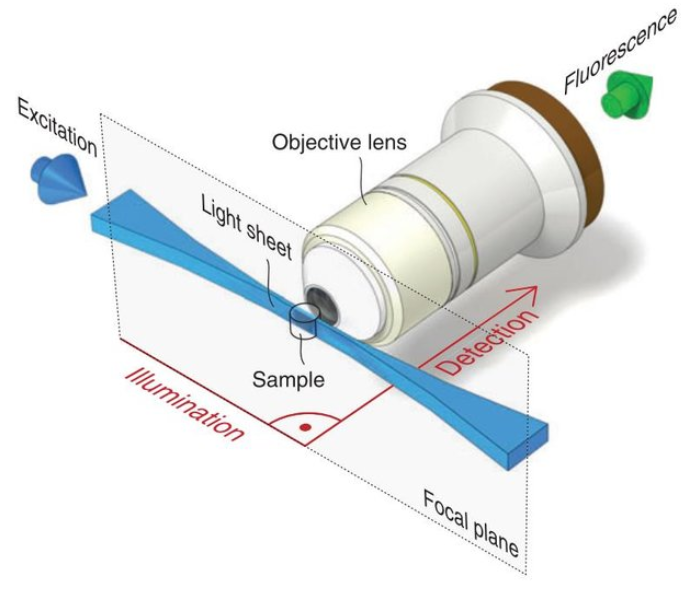
The main characteristic of the LSFM is that illuminates the specimen with thin light sheets, plane by plane, leading to optical sectioning. This approach reduces light exposure and, in consequence, photo-toxicity and photo-bleaching are trimmed down as opposed to other fluorescence microscopes. The latter allows long periods of time for acquisition among other benefits that make the LSFM one of the preferred techniques for 3D imaging of big specimens. As a result, this procedure gives a stack of 2D images along the direction of detection. However, as with almost every optical phenomena, it presents problems such as blurring, and shadows as the laser goes through the object. One of the reasons for this is the scattering that photons suffer, exciting fluorophores not only in the focal plane but also in close-plane. Hence, we want to reconstruct the fluorophore distribution from the images of the microscope, for which an inverse problem is established.

Thus, the direct model is divided into two steps: illumination or excitation and projection or fluorescence. A PDE describing the photon distribution is used for each step obtaining an explicit formula that shall be related to the solution of the heat equation in $\mathbb{R}$.

The model

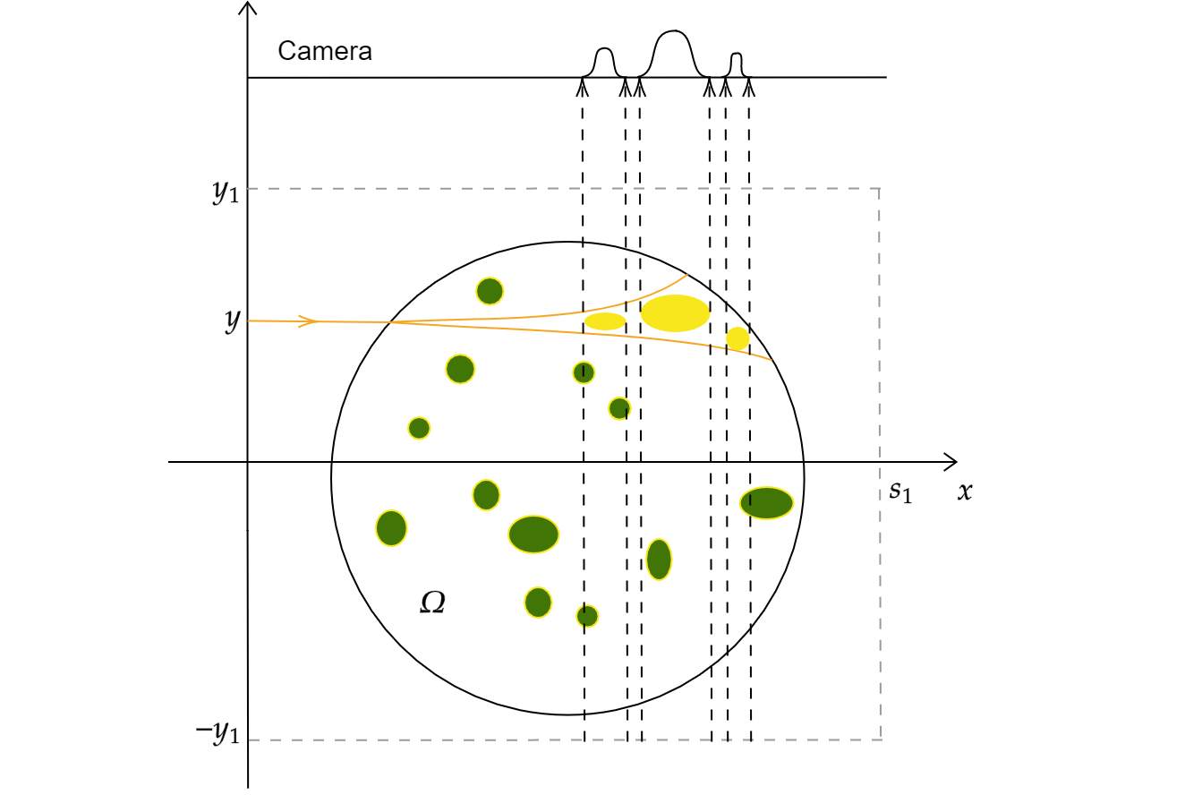
As a first idea, a 2D model is set, so, instead of considering a 3D specimen, we illuminate a 2D object and, instead of illuminating plane by plane, we illuminate lines or fibres of the specimen emitting laser beams at different heights. To move from this 2D model to the 3D one, the plane illumination shall be modelled with a collection of laser beams.

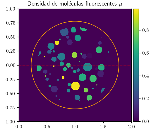
In what follows, the fluorophore distribution shall be denoted $\mu$ and will be the unknown for the inverse problem. An example of this function is given in the next figure:

Illumination step. Fermi pencil-beam equation.

For the illumination step, it is considered the Fermi pencil-beam equation, which describes the transport of photons in a highly scattering and highly peaked forward regime when emitted from height $y=0$. The equation is as follows:

$$\{\begin{array}{l}\begin{array}{rcl}({\partial }_x+{\theta }_y{\partial }_y+\lambda (x,h)-\psi (x,h){\partial }_{{\theta }_y}^2)u(x,y,{\theta }_y)& =& 0\\ u(x_h,y,{\theta }_y)& =& {\delta }_h(y){\delta }_0({\theta }_y)\\ x\in (x_h,\mathrm{\infty }),y\in \mathbb{R},{\theta }_y\in \mathbb{R}& & \end{array}\end{array}$$

But we are interested in the function $v_h(x,y)$ that describes the photon distribution independent of the angle ${\theta }_y$:

$$\begin{array}{rcl}{v}_h(x,y)& =& {\displaystyle {\int }_{\mathbb{R}}u(x,y,{\theta }_y)d{\theta }_y}\\ & =& \text{exp}(-{\displaystyle {\int }_{x_h}^x\lambda (\tau ,h)d\tau }){\displaystyle \frac{1}{\alpha (x,h)\sqrt{2\pi }}}\text{exp}(-{\displaystyle \frac{(y-h{)}^2}{2{\alpha }^2(x,h)}})\end{array}$$

Hence, the fluorescent source $w_h(x,y)$ (that is, the fluorophores that have been excited) is given by

$$w_h(x,y)=c\cdot \mu (x,y)\cdot v_h(x,y)$$

Fluorescence step. Radiative transfer equation.

Fluorophores excited will now be able to emit fluorescent light. Let $p_h(x,\theta )$ be the intensity of photons at point $x$ moving along the direction $\theta$ and coming from fluorophores when illuminating at height $h$. We consider that the transport of photons is governed by a linear transport equation with attenuation $a$ and source $w_h$:

$$\{\begin{array}{l}\begin{array}{rl}\theta \cdot {\mathrm{\nabla }}_{x,y}{p}_h(x,y,\theta )+a(x,y)p_h(x,y,\theta )=w_h(x,y),& \mathrm{\forall }(x,y)\in {\mathbb{R}}^2,\theta \in {\mathbb{S}}^1\\ {\displaystyle \underset{t\to \mathrm{\infty }}{lim}{p}_h((x,y)-t\theta ,\theta )=0,}& \mathrm{\forall }(x,y)\in {\mathbb{R}}^2,\theta \in {\mathbb{S}}^1\end{array}\end{array}$$

The boundary condition states that there are no external sources. There exists a unique solution for this equation:

$$p_h(x,y,\mathit{\theta })={\displaystyle {\int }_{-\mathrm{\infty }}^0{w}_h((x,y)+r\mathit{\theta })\text{exp}(-{\displaystyle {\int }_r^{0}a((x,y)+\tau \mathit{\theta })d\tau })dr}$$

We are interested in what is measured in pixel $s$ and, also, we assume that cameras are collimated. Hence, the final measurement obtained at pixel $s$ when illuminating at height $h$ is given by the next expression:

$$\begin{array}{rcl}p(s,h)& =& c\cdot \text{exp}(-{\displaystyle {\int }_{x_h}^s\lambda (\tau ,h)d\tau })\cdot \\ & & {\displaystyle {\int }_{-\mathrm{\infty }}^{\mathrm{\infty }}{\displaystyle \frac{\mu (s,r)e^{-{\int }_r^{\mathrm{\infty }}a(s,\tau )d\tau }}{\alpha (s,h)\sqrt{2\pi }}}\text{exp}(-{\displaystyle \frac{(r-h{)}^2}{2{\alpha }^2(s,h)}})dr}\end{array}$$

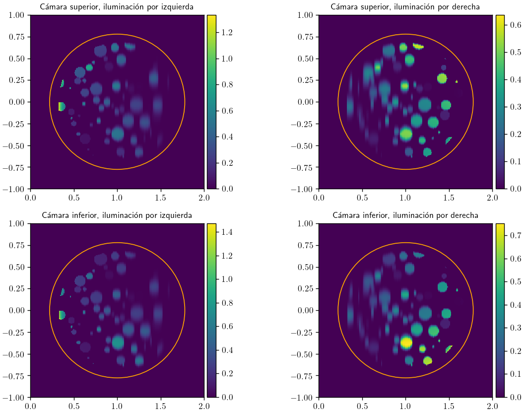
An example for measurements obtained when illuminating by left and right the source in figure 2 and measuring with upper and lower cameras is given in the next figure:

The inverse problem and the heat equation.

The inverse problem consists of reconstructing the fluorophore distribution $\mu$ from measurements $p(s,h)$. We suppose as known the functions $\lambda$, $a$ and $\psi$. The latter function may be seen as the convolution of $\mu (s,\cdot )\cdot e^{-{\int }_{\cdot }a(s,\tau )d\tau }$ with the heat kernel. In fact, let $s$ fixed and define

$$\begin{array}{rcl}\sigma (y)& :=& {\displaystyle \frac{1}{2}}{\alpha }^2(s,y)={\displaystyle \frac{1}{2}}{\displaystyle {\int }_{x_h}^s(s-\tau {)}^2\psi (\tau ,y)d\tau }\\ f(r)& :=& \mu (s,r)\text{exp}(-{\displaystyle {\int }_r^{\mathrm{\infty }}a(s,\tau )d\tau })\\ g(y)& :=& {\displaystyle \frac{1}{c}}p(s,y)\text{exp}\left({\displaystyle {\int }_{x_h}^s\lambda (\tau ,y)d\tau }\right)\end{array}$$ hence, $$g(y)={\displaystyle {\int }_{\mathbb{R}}{\displaystyle \frac{f(r)}{\sqrt{4\pi \sigma (y)}}}\text{exp}(-{\displaystyle \frac{(r-y{)}^2}{4\sigma (y)}})}$$

Thus, considering the heat equation in $\mathbb{R}$:

$$\{\begin{array}{l}\begin{array}{rcll}{u}_t-u_{yy}& =& 0,& (y,t)\in \mathbb{R}\times (0,+\mathrm{\infty }),\\ u(y,0)& =& f(y),& \text{si }y\in Y_s,\\ u(y,0)& =& 0,& \text{si }y\notin Y_s,\\ {\displaystyle \underset{|y|\to \mathrm{\infty }}{lim}u(y,t)}& =& 0,& \mathrm{\forall }t>0\end{array}\end{array}$$

we have

$$u(y,\sigma (y))={\displaystyle {\int }_{\mathbb{R}}{\displaystyle \frac{f(r)}{\sqrt{4\pi \sigma (y)}}}\text{exp}(-{\displaystyle \frac{(y-r{)}^2}{4\sigma (y)}})dr=g(y)}$$

That is, we can see $g$ as the measurements or available information, $f$ is the initial condition related to our unknown $\mu$ and $\sigma$ may be related to the time variable for the heat kernel. Thus

The fluorophore distribution $\mu$ is related to the initial condition of the heat equation.

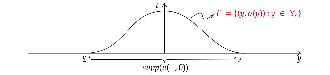
Observations of $u$ are available on the curve $\mathrm{\Gamma }:=(y,\sigma (y)):y\in Y_s\subseteq \mathbb{R}\times [0,+\mathrm{\infty })$, which turns out to have the following form:

Uniqueness of the inverse problem

By linearity, the uniqueness of the inverse problem is reduced to an injectivity result:

Theorem. Let $s$ be fixed. If $p(s,y)=0$ $\mathrm{\forall }y\in Y_s$, then $\mu (s,y)=0$ $\mathrm{\forall }y\in Y_s$.

But this result is a direct consequence of a uniqueness result for the heat equation:

Theorem. Let $\sigma \in C_c^1(\mathbb{R})$ and $\mathrm{\Gamma }=(t,y)\in {\mathbb{R}}^2:t=\sigma (y)$. Let $\underset{―}{y}=inf(supp(\sigma ))$ and $\bar{y}=sup(supp(\sigma ))$. Assume that there exists $\delta >0$ such that ${\sigma }^{\prime }(y)>0$ in $(\underset{―}{y},\underset{―}{y}+\delta )$. Hence, if $u\equiv 0$ on $\mathrm{\Gamma }$, then $u(\cdot ,0)\equiv 0$.

Stability of the inverse problem

A stronger (but harder) result than uniqueness is stability, which asks for the continuity of the inverse operator, that is if small changes in measurements lead to small changes in the respective fluorophore distributions. From the numerical point of view, stability is a critical point since mathematical models do not represent reality in a perfect way and the instruments used to measure may present noise. Thus, if the problem is not stable, the reconstructed solution may present huge differences from the original solution.

First, a logarithmic stability result is presented. This kind of estimate is undesirable since small changes in measurements may lead to large errors in the reconstruction. For this estimate, we add some apriori information supposing that the solution $u_0$ belongs to a bounded set of a fractional Sobolev space.

Theorem. Let $0<\beta <1$. Let $u$ be the solution of the heat equation in ${\mathbb{R}}^n$ with $u_0\in \mathcal{A}:=\{a\in H^{2\beta }({\mathbb{R}}^n);||a|{|}_{H^{2\beta }({\mathbb{R}}^n)}\le M\}$. Let $0\le \tau <T$ and $\omega \subset {\mathbb{R}}^n$ be an open set with bounded complement such that $\omega \times (\tau ,T)$ is the observation set. If $||u|{|}_{L^2(\omega \times (\tau ,T))}<1$, then for every $0<\epsilon <(T-\tau )/2$, $\delta >0$ and $\theta \in (\tau +\epsilon ,T-\epsilon )$ there exist constants $\kappa =\kappa (\beta )\in (0,1)$ and $C=C(\epsilon ,\delta ,M,\theta )>0$ such that $$||u_0|{|}_{L^2({\mathbb{R}}^n)}\le C{(-log||u|{|}_{L^2(\omega \times (\tau ,T))})}^{-\kappa }$$

The previous theorem would allow us to conclude a logarithmic-type stability for the LSFM inverse problem. However, there is a hypothesis that may improve the result, which is that in the LSFM model, the initial condition is compactly supported. This additional hypothesis gives a Lipschitz-type stability result:

Theorem. For $R>0$ we define $B:=B(0,R)$ the ball of radius $R$ and centered at the origin. Let $0\le \tau <T$ and $\omega \subseteq {\mathbb{R}}^n$ be such that ${\mathbb{R}}^n\mathrm{\setminus }\omega$ is compact and $B\subseteq {\mathbb{R}}^n\mathrm{\setminus }\omega$. Let $u_0\in L^1({\mathbb{R}}^n)$ be with $supp(u_0)\subseteq B$ and $u$ be the respective solution of the heat equation. Then there exists a constant $C=C(R,\tau ,T,\omega )>0$ such that $$||u_0|{|}_{L^1({\mathbb{R}}^n)}\le C||u|{|}_{L^2(\omega \times (\tau ,T))}$$